
EVN User Experiment Pipeline Feedback
Last updated: Fri Apr 21 15:31:00 CEST 2017
burns@jive.eu
General Comments.
(
Brief data summary
and
scan listing
)
EL058B, C-band eVLBI experiment on 17 April 2017, Participating stations: Mc, Ib, Jb, Mc, Nt, O8, Tr, Ys, Wb, Hh You can find information on individual stations at: http://www.evlbi.org/user_guide/EVNstatus.txt.
The following are plots from the EVN pipeline analysis, in which the refant was: Ys
The EVN reliability indicator (ERI) for stations in this experiment were
Plots of the autocorrelations
Comments.
Auto-corr Amplitude vs frequency plots for each station showing all IFs and Pols. RFI can easily be found by looking at the continuum source scans in this plot.
Plots of the uncalibrated amplitude and phase
against time
Comments.
Amp and phase vs time, for the whole experiment. Shows visibilities on all baselines to the refant. All IFs and Pols shown. This is a good place to look for stations that missed scans during the experiment.
The first few pages look alarming for Jb, Tr and Wb - with their lack of good data, however this is expected since these stations only use 4 BBCs of each Pol; They dont have IFs 1-4. If you look at page 25 onwards you can see IFs 5 onwards which show good data for these stations. No problems here. Onsala data were actually unusable due to there being an issue with the polar drive motor.
Plots of the uncalibrated amplitude and phase
against frequency channel
Comments.
Uncalibrated, vector averaged, cross power specra for baselines to the refant. No bandpass done yet. This is a good place to look check how well detected sources are on each baseline.
Fringes look good. Again, the missing IFs of Jb, Wb and Tr are as expected from their data transfer settings.
The uncalibrated amplitude and phase of the crosshand
correlations against frequency channel
Comments.
TSYS against time
Comments.
Plots of system temperature vs time for each station (and each IF). Flat-line plots indicate that this information was not available for a given station, in which case we create a generic tsys table scalled to the station's gain (Jy/K).
Telescope sensitivities
from the a priori TSYS and Gain
curves (the square of this number gives the antenna noise (SEFD) in Jy - the
smaller the better).
Comments.
Gain info in CL2, determined using tsys tables. Plot shows Gain vs time for each station, each IF and each Pol.
Fringe-fit phase solutions
(including Parallactic
Angle correction).
Comments.
Pot of CL3. This is the CL table generated using CL2 (amplitude cal) and SN2 (FRING solutions). Plot shows phase calibration data vs time. Missing data indicate possible issues in those previous steps. If the data are complete (all stations and most scans present) then use this table to phase-reference the target.
Fringe-fit delay solutions
Comments.
Plot of SN2. Shows delay vs time from FRING results (usually only calibrators and reference sources). This is a good place to look for times where FRING failed to get solutions. Here FRING uses a signal to noise cutoff of 7.
Fringe-fit rate solutions
Comments.
SN2 as abover, but for rate.
Telescope bandpasses
Comments.
Plot of BP1; the bandpass characteristic of each station, determined using the brightest source(s) in the experiment. Look for small dispersion in the phase data, this indicates a high signal to noise - which will lead to better bandpass characterisation.
Nice!
Calibrated amplitude and phase against time
(a
priori amplitude calibration and fringe-fit solutions applied).
Comments.
Plot of visibilities vs time for all baselines to the refant, after applying CL3. This is a good place to look for quickly checking the success of the antab (CL2) and FRING (CL3) stages of the pipeline.
Again, as above, Jb, Tr, Wb appear from pg25 onwards (IF 5 onwards)
Calibrated amplitude and phase against frequency
channel
Comments.
Amp and phas vs frequency plots for all baselines to refant, after applying CL3 and BP1. If CL3 and BP1 are good you will get flat phase and amplitude profiles, therefore this is a good place to check the success of CL2 and particluarly BP1 for each scan/baseline/IF/Pol.
Naturally weighted dirty map (not useful for bright sources)
produced before self-cal of:
OQ208: pdf (not available)
, or
FITS (not available)
.
ARSCO:
pdf
, or
FITS
.
J1625-2527: pdf (not available)
, or
FITS (not available)
.
J1621-2241:
pdf
, or
FITS
.
Comments.
Naturally-weighted dirty maps of phase-referenced targets.
Uniformly weighted dirty map (not useful for bright sources)
produced before self-cal of:
OQ208: pdf (not available)
, or
FITS (not available)
.
ARSCO:
pdf
, or
FITS
.
J1625-2527: pdf (not available)
, or
FITS (not available)
.
J1621-2241:
pdf
, or
FITS
.
Comments.
Uniformly-weighted dirty maps of phase-referenced targets.
Phase corrections applied to a priori calibrated and
fringe-fitted data by self-calibration.
OQ208
.
ARSCO (not available)
.
J1625-2527
.
J1621-2241 (not available)
.
Comments.
Individual plots for each source that was used in FRING. Shows phase selfcal solutions (SN1 after SPLIT). This is particularly useful to check if the reference source could be self-calibrated, and to look for missing scans/antennae.
Amplitude corrections applied to a priori calibrated and
fringe-fitted data by self-calibration.
OQ208:
pdf
, or
text file
, or
statistical summary
.
ARSCO: pdf (not available)
, or
text file (not available)
, or
statistical summary (not available)
.
J1625-2527:
pdf
, or
text file
, or
statistical summary
.
J1621-2241: pdf (not available)
, or
text file (not available)
, or
statistical summary (not available)
.
Comments.
Individual plots for each source that was used in FRING. Shows amplitude selfcal solutions (SN2). This table is important to properly calibrate amplitudes from stations that had to use generic tsys tables (see TSYS, above).
Telescope sensitivities
(the total AMP gain applied
during both a priori and self calibration; the square of this number gives the
antenna noise (SEFD) in Jy).
Comments.
Plot of CL4 which shows amplitude calirations determined from CL3 and the amplitude selfcal solutions from SN2 (from CALIB_AMP2, above). Comparison with GAIN plot (above) reveals the accuracy of the apriori amplitude calibration derived from the TSYS tables - this is particularly important for stations that have generic generated TSYS tables; Tsys may benefit from aditional scalling if there is a large differnce in SENS and GAIN plots.
Residual closure phase (visibility closure phase with model closure phase subtracted) for:
OQ208
.
ARSCO (not available)
.
J1625-2527
.
J1621-2241 (not available)
.
Comments.
Closure phases for all triangles of antennae in the array. Individual plots for each source which was used in FRING.
Calibrated visibilities and the source model of:
OQ208
.
ARSCO (not available)
.
J1625-2527
.
J1621-2241 (not available)
.
Comments.
Similar to VPLOT_CAL for sources used in FRING, however each source has been individually SPLITed and modelled.
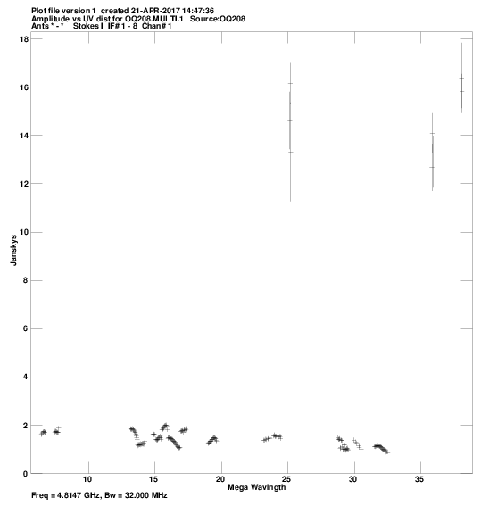
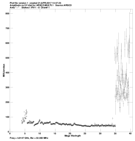
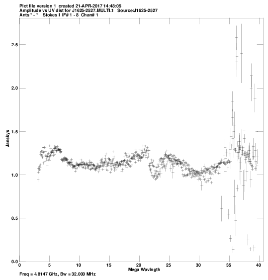
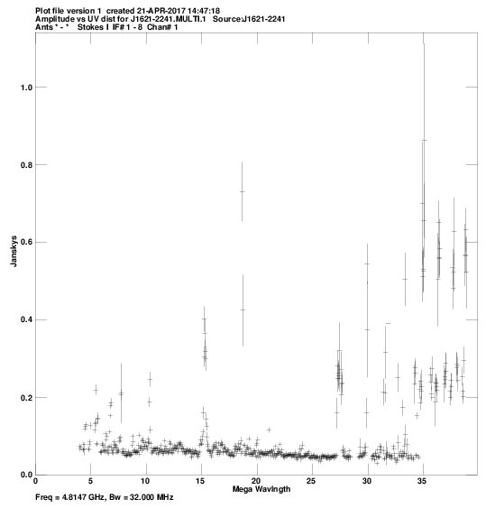
Calibrated visibilities against u,v distance for:
OQ208:
pdf
, or
png
.
ARSCO:
pdf
, or
png
.
J1625-2527:
pdf
, or
png
.
J1621-2241:
pdf
, or
png
.
Comments.
Plot of amplitude vs baseline lenght for each source. This can be useful to look for inications of structure at different angular scales.
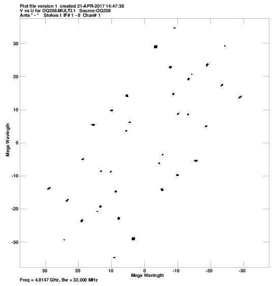
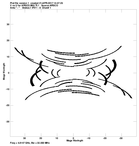
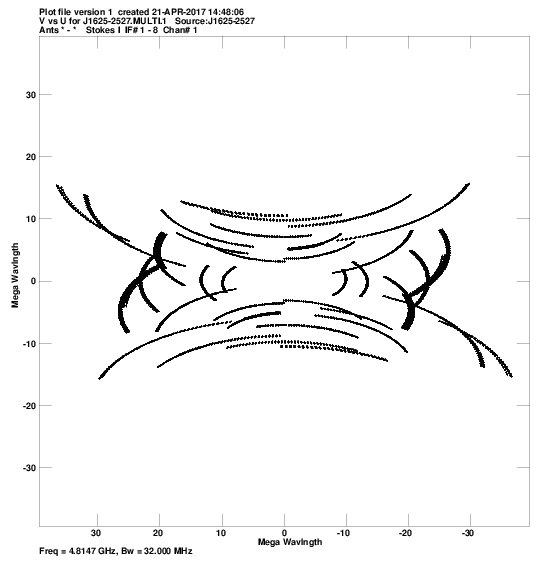
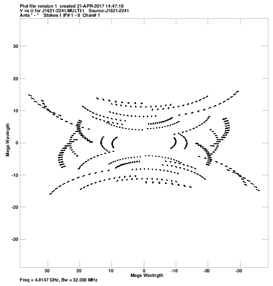
u,v coverage for:
OQ208:
pdf
, or
png
.
ARSCO:
pdf
, or
png
.
J1625-2527:
pdf
, or
png
.
J1621-2241:
pdf
, or
png
.
Comments.
Plot of the UV coverage for each source during the experiment.
Crude maps of sources:
OQ208:
pdf
, or
FITS
.
ARSCO:
pdf
, or
FITS
.
J1625-2527:
pdf
, or
FITS
.
J1621-2241:
pdf
, or
FITS
.
Comments.
CLEANed image of each source (FRINGed or phase-referened) after applying all relevant calibration by the pipeline up to CL4; amplitude and phase selfcal calibrations.