
EVN User Experiment Pipeline Feedback
Last updated: Wed Nov 16 16:18:58 CET 2022
orosz@jive.eu
General Comments.
(
Brief data summary
and
scan listing
)
EB081B. L-band experiment observed on 04 November 2020. This is a continuum pass dataset.
The data rate was 1024 Mbps (8 x 16 MHz subbands, full polarization, two-bit sampling)
The target source ROSS867 was calibrated using the phase-reference source J1722+2458.
3C345 and OQ208 were also observed as calibrators and fringe finders.
16 stations participated: Jl, Jb, Wb, Ef, Mc, Nt, O8, T6, Ur, Tr, Hh, Sv, Zc, Bd, Ir, Sr.
The following are plots from the EVN pipeline analysis, in which the reference antenna was: Ef.
Plots of the autocorrelations
Comments.
Auto-corr amplitude vs frequency plots for each station showing all IFs and Pols.
Plots of the uncalibrated amplitude and phase
against time
Comments.
Amplitude and phase vs time, for the whole experiment, no calibration applied. Shows visibilities on all baselines to the reference antenna. All IFs and Pols shown. This is a good place to look for stations that missed scans during the experiment.
Plots of the uncalibrated amplitude and phase
against frequency channel
Comments.
Uncalibrated, vector averaged, cross power specra for baselines to the reference antenna. No bandpass calibration applied yet. This is a good place to check how well detected sources are on each baseline.
The uncalibrated amplitude and phase of the crosshand
correlations against frequency channel
Comments.
TSYS against time
Comments.
Plots of system temperature vs time for each station (and each IF). Flat-line plots indicate that this information was not available for a given station, in which case we create a generic Tsys table scaled to the station's gain (Jy/K). This information is stored in the TY1 table.
Telescope sensitivities
from the a priori TSYS and Gain
curves (the square of this number gives the antenna noise (SEFD) in Jy - the
smaller the better).
Comments.
Gain info in CL2, determined using Tsys tables. Plot shows Gain vs time for each station, each IF and each Pol.
Fringe-fit phase solutions
(including Parallactic
Angle correction).
Comments.
Plot of CL4. This is the CL table generated using CL3 (amplitude cal and primary beam corrections if required) and SN3 (FRING solutions). Plot shows phase calibration data vs time. Missing data indicate possible issues in those previous steps. If no issues arose, then use this table to phase-reference the target.
Fringe-fit delay solutions
Comments.
Plot of SN3. Shows delay vs time from FRING results (usually only calibrators and reference sources). This is a good place to look for times where FRING failed to get solutions. Here, FRING uses a signal to noise cutoff of 7.
Fringe-fit rate solutions
Comments.
SN3 as above, but for rate.
Telescope bandpasses
Comments.
Plot of BP1. Shows the bandpass characteristics of each antenna, determined using the brightest source(s) in the experiment. Look for small dispersion in the phase data, this indicates a high signal to noise ratio - and thus a good bandpass characterisation.
Calibrated amplitude and phase against time
(a
priori amplitude calibration and fringe-fit solutions applied).
Comments.
Plot of visibilities vs time for all baselines to the reference antenna, after applying CL4. This is a good place to check the success of the amplitude calibration (CL2) and primary beam correction (CL3) and FRING (CL4) stages of the pipeline.
Calibrated amplitude and phase against frequency
channel
Comments.
Amplitude and phase vs frequency plots for all baselines to the reference antenna, after applying CL4 and BP1. If the corrections of CL2, CL4 and BP1 are good enough, you will get flat phase and amplitude profiles, therefore this is a good place to check the success of CL3, CL4 and particularly BP1 for each scan/baseline/IF/Pol.
Naturally weighted dirty map (not useful for bright sources)
produced before self-cal of:
J1800+3848: pdf (not available)
, or
FITS (not available)
.
J1722+2458: pdf (not available)
, or
FITS (not available)
.
J1722+2815: pdf (not available)
, or
FITS (not available)
.
OQ208: pdf (not available)
, or
FITS (not available)
.
3C345: pdf (not available)
, or
FITS (not available)
.
J1716+2616: pdf (not available)
, or
FITS (not available)
.
ROSS867:
pdf
, or
FITS
.
Comments.
Only phase-referenced targets are shown.
Uniformly weighted dirty map (not useful for bright sources)
produced before self-cal of:
J1800+3848: pdf (not available)
, or
FITS (not available)
.
J1722+2458: pdf (not available)
, or
FITS (not available)
.
J1722+2815: pdf (not available)
, or
FITS (not available)
.
OQ208: pdf (not available)
, or
FITS (not available)
.
3C345: pdf (not available)
, or
FITS (not available)
.
J1716+2616: pdf (not available)
, or
FITS (not available)
.
ROSS867:
pdf
, or
FITS
.
Comments.
Only phase-referenced targets are shown.
Phase corrections applied to a priori calibrated and
fringe-fitted data by self-calibration.
J1800+3848
.
J1722+2458
.
J1722+2815
.
OQ208
.
3C345
.
J1716+2616
.
ROSS867 (not available)
.
Comments.
Individual plots for each source that was used in FRING. Shows phase selfcal solutions (SN1 after SPLIT). This is particularly useful to check if the reference source could be self-calibrated, and to look for missing scans/antennas.
Amplitude corrections applied to a priori calibrated and
fringe-fitted data by self-calibration.
J1800+3848:
pdf
, or
text file
, or
statistical summary
.
J1722+2458:
pdf
, or
text file
, or
statistical summary
.
J1722+2815:
pdf
, or
text file
, or
statistical summary
.
OQ208:
pdf
, or
text file
, or
statistical summary
.
3C345:
pdf
, or
text file
, or
statistical summary
.
J1716+2616:
pdf
, or
text file
, or
statistical summary
.
ROSS867: pdf (not available)
, or
text file (not available)
, or
statistical summary (not available)
.
Comments.
Individual plots for each source that was used in FRING. Shows amplitude selfcal solutions (SN3). This table is important to properly calibrate amplitudes from stations that had to use generic Tsys tables (see TSYS, above). In the statistical summary, values close to one mean a good a-priori calibration.
Telescope sensitivities
(the total AMP gain applied
during both a priori and self calibration; the square of this number gives the
antenna noise (SEFD) in Jy).
Comments.
Plot of CL5 which shows amplitude calibrations determined from CL4 and the amplitude selfcal solutions from SN3 (from CALIB_AMP2, above). Comparison with GAIN plot (above) reveals the accuracy of the apriori amplitude calibration derived from the TSYS tables - this is particularly important for stations that have generic generated TSYS tables; Tsys may benefit from additional scaling if there is a large difference in SENS and GAIN plots.
Residual closure phase (visibility closure phase with model closure phase subtracted) for:
J1800+3848
.
J1722+2458
.
J1722+2815
.
OQ208
.
3C345
.
J1716+2616
.
ROSS867 (not available)
.
Comments.
Closure phases for all triangles of antennas in the array. Individual plots for each source that was used in FRING.
Calibrated visibilities and the source model of:
J1800+3848
.
J1722+2458
.
J1722+2815
.
OQ208
.
3C345
.
J1716+2616
.
ROSS867 (not available)
.
Comments.
Similar to VPLOT_CAL for sources used in FRING, however, each source has been individually SPLITed and modelled.
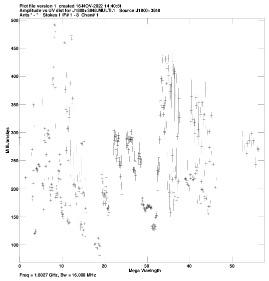
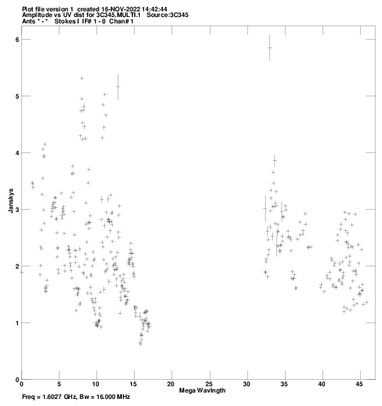
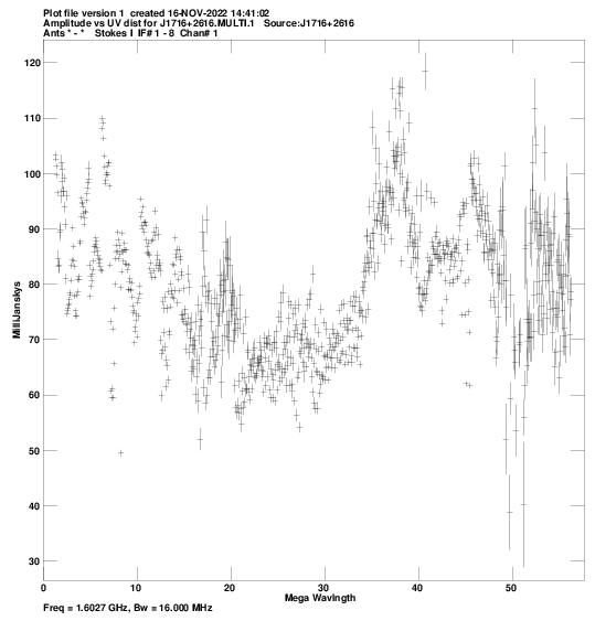
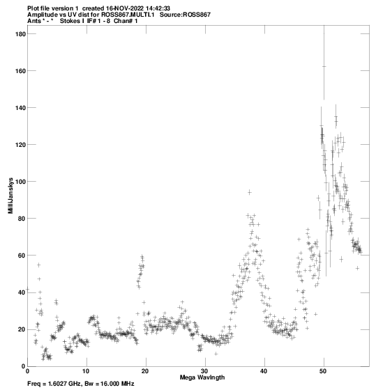
Calibrated visibilities against u,v distance for:
J1800+3848:
pdf
, or
png
.
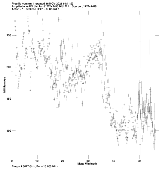
J1722+2458:
pdf
, or
png
.
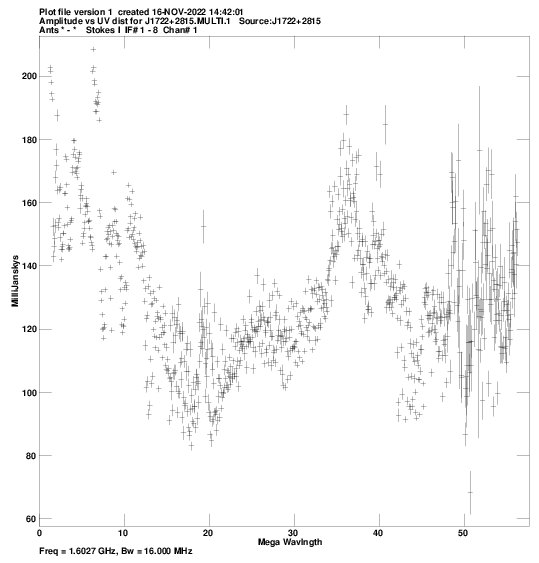
J1722+2815:
pdf
, or
png
.
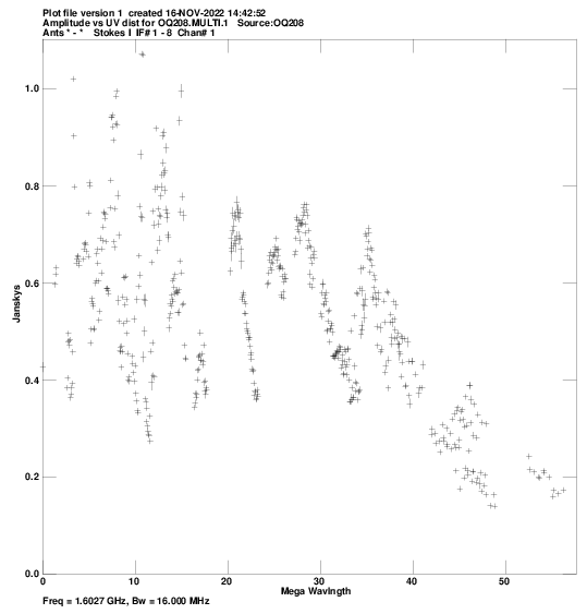
OQ208:
pdf
, or
png
.
3C345:
pdf
, or
png
.
J1716+2616:
pdf
, or
png
.
ROSS867:
pdf
, or
png
.
Comments.
Plot of amplitude vs baseline length for each source. This can be useful to look for indications of structure at different angular scales.
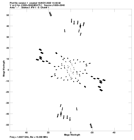
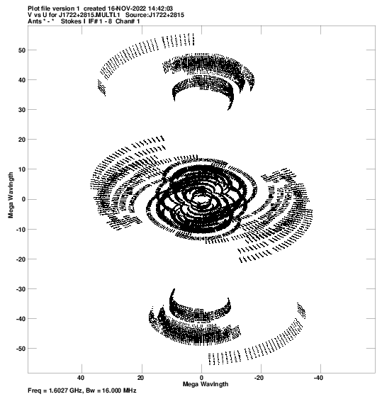
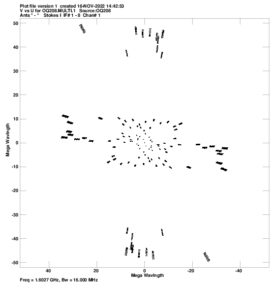
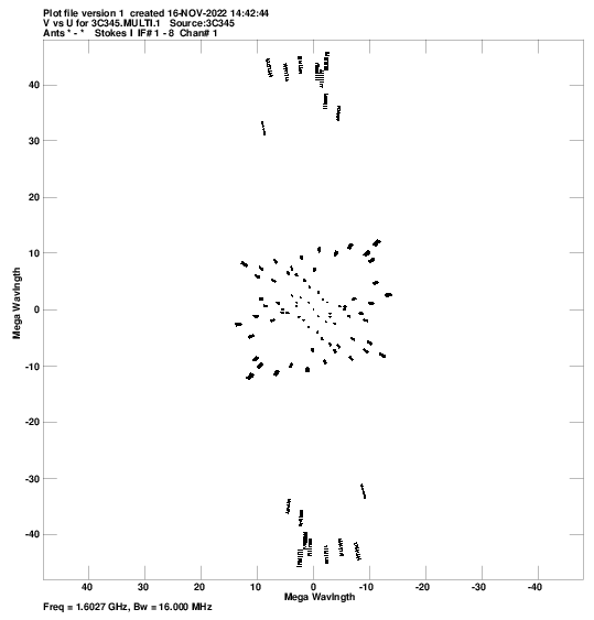
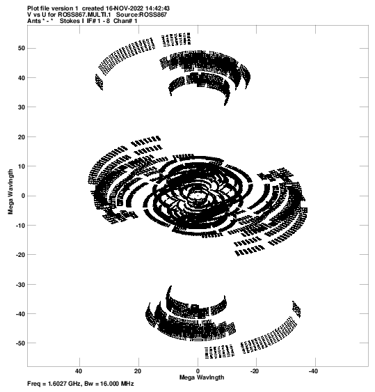
u,v coverage for:
J1800+3848:
pdf
, or
png
.
J1722+2458:
pdf
, or
png
.
J1722+2815:
pdf
, or
png
.
OQ208:
pdf
, or
png
.
3C345:
pdf
, or
png
.
J1716+2616:
pdf
, or
png
.
ROSS867:
pdf
, or
png
.
Comments.
Plot of the UV coverage for each source during the experiment.
Crude maps of sources:
J1800+3848:
pdf
, or
FITS
.
J1722+2458:
pdf
, or
FITS
.
J1722+2815:
pdf
, or
FITS
.
OQ208:
pdf
, or
FITS
.
3C345:
pdf
, or
FITS
.
J1716+2616:
pdf
, or
FITS
.
ROSS867:
pdf
, or
FITS
.
Comments.
CLEANed image of each source (FRINGed or phase-referenced) after applying all relevant calibrations up to CL5 by the pipeline; including amplitude and phase self calibrations.